Wavelets have become a hot topic in mathematics in general and computer graphics in particular. They are a useful tool for multiresolution analysis of a data set and for data compression. There are several popular wavelet basis and scaling functions. Herein I will focus on the Haar wavelet basis and its application to compression of low contrast textures in a 3d polygonal game engine that I am developing. In this application, I exploit both of these characteristics of the Haar basis.
## Terminology
For the purposes of this article, a texture consists of a 32 bit image, 2n texels wide, 2n texels tall. A texel is an industry buzzword for a pixel of the texture before it is projected onto the screen. Mipmaps are also stored for each image. Each mipmap is a power of two smaller than the last and is generated by antialiasing from the previous image. So the mipmap set for a 128x128 texture would be 64x64, 32x32, 16x16,8x8,4x4,2x2 and 1x1. Typically, the lowest 3 or 4 mipmap levels are more hassle to maintain than they are worth and are often omitted since for a game one can often constrain the scene to keep polygons that are that far away from being visible. Also, if they are visible, you probably have bigger problems with the sheer number of small polygons you need to project and display than worrying about a little aliasing problem in the distance. Storing the mipmaps drives up texture storage requirements by 1/3rd.
## The Problem
A typical texture size is 256x256. At 4 bytes per texel this single image consumes 256Kb of RAM per texture. A practical scene has approximately a dozen textures visible at a time, and up to a hundred distributed around the map in places where they are not immediately visible. To keep everything loaded at all times would require approximately 200Mb of memory just for the texture and mipmap data, let alone any game logic, lightmapping or geometry. Needless to say, at this time expecting that much memory from a typical end user's i computer is unreasonable.
## Possible Solutions
One solution is to reduce the images to 8 bit palettized representations. This reduces memory requirements to about 50Mb, which can be reasonably swapped to and from disk if you can exploit coherence in the way textures are distributed around the map. However, if you cannot take advantage of any spatial coherence or caching then you will experience a stutter caused by the sudden hit of having to go look up the texture to continue rendering the display. This stutter has a very negative psychological effect; As a player, you are suddenly reminded that you are playing a game and the sense of immersion goes out the window. Frame rate consistency is more important over all than the best case performance, so a performance leveling factor is required. The stutter is aggravated by the fact that in order to swap textures the engine has to look to disk, which is several orders of magnitude slower than accessing the texture directly from memory. Also, a paletted representation of textures requires you to use a smaller subset of colorspace to store the image, you tend to lose a lot of quality in the conversion, and even reconstructed, if you are using a standard palette with six bit color components, the reconstructed texel is at best 18 bits upon reconstruction. Other complications arise when you want to store an alpha (translucency) channel in a paletted representation.
Another option is to store a compressed representation of the texture in memory and to derive the mipmaps from that. The problem with this approach is that you are stuck decompressing the entire texture and then extracting all mipmap levels even if you only needed the 32x32 mipmap from a 256x256 texture. Typically, you will need the lower mipmaps before the larger mipmaps for a given texture. This is intuitive since as you walk through a scene, surfaces will come into view in the distance and get closer. As they approach, they will gradually need more detail (higher mipmap levels). With this approach you have to take the full hit all at once. This introduces stutter. JPEG style compression can be used to good effect, you can typically obtain a higher compression ratio than by using the approach I took below. Unfortunately, its all or nothing nature makes it ill suited to my needs. Also, the better compression comes at the cost of having to perform the inverse DCT on each 8x8 block of the image. This process takes 54 multiplications, 462 additions and 6 shifts per channel using Feig's method, which is presently the most efficient published method on Intel processors. In comparison the same 8x8 block decompresses with 256 additions per channel using Haar.
## An overview of the Haar Basis
This is intended to supply an intuitive understanding of how the Haar basis works. What follows is not intended as a rigorous mathematical proof or examination of the subject.
```text
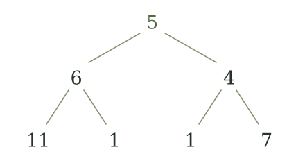
Given 2^n samples such as: { 11, 1, 1, 7 }
Pair samples and average them giving: { (11+1)/2, (1+7)/2 } = { 6, 4 }
Repeat until you have 1 value: { (6+4)/2 } = { 5 }
```
Figure 1. Pairwise averages and the scaling value.
This value at the top of this tree (Figure 1) is your scaling value.
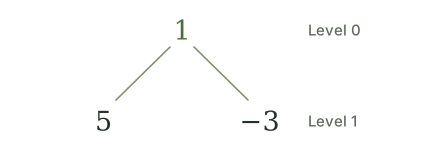
Now, you recurse down the hierarchy that you paired. At each level you subtract value in the right hand child of the current node from the value in the current node. Do not recurse into the leaf nodes on the tree.
Figure 2. Wavelet coefficients by level.
There are 2n values in a given level of the tree. These values are your wavelet coefficients. With these values you can reconstruct the original sample set since this operation is invertible.
There are 2m coefficients at the mth level of the hierarchy. Adding the scaling value to this set, provides the sample number of values as the original data set, however when converted into Haar form, the numbers are now indicative of the changes from the smaller level.
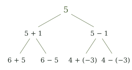
Reconstruction is straightforward. Start with the scaling value and the coefficient for level 0. Add the coefficient to the scaling value to generate the left hand child, subtract it from the scaling value to generate the right hand child. Take those nodes and repeat down the tree:
=
Figure 3. Reconstruction: add on the left, subtract on the right.
Next you weight the coefficients by their level in the tree. This is don't to normalize the coefficients. There are several weighting mechanisms that are popular. Each of them is valid for a different uses. I prefer normalization by multiplying each value by 1/sqrt(2^j) where j is the coefficient's level in the tree.
Your data now to consists of:
```text
The scaling value { 6 }
The wavelet coefficients { 1, 5, -3}
The weighted wavelet coefficients { 1, 5/sqrt(2), -3/sqrt(2) }
```
So far, no compression has resulted from this process. The entire transformation merely converted four values into four other values and some weighted values which are derived from them.
## Applying Haar
The next step is to figure out how to apply this to image compression. An image is a two dimensional grid of samples, not a one dimensional set as mentioned above.
There are two common approaches:
The standard decomposition of the image would perform the Haar transform on each row and then goes through column by column and transforms each in turn. This unfortunately is not very useful for reconstructing mipmaps, since in order to extract a 2x2 mipmap, I would need to reconstruct the entire image, and then anti-alias my way back down to 2x2. If I were to do this, there would be no advantage in reconstructing the lower mipmaps.
The nonstandard decomposition transforms one level down each row, and then transforms one level down each column, and repeats until you are left with the scaling function. Thus intuitively, you can extract a 2x2 mipmap from the 1x1 mipmap (aka your scaling coefficient) and the set of coefficients for level 0 (one row coefficient and two column coefficients) and then extract the 4x4 mipmap from the 2x2 using the mipmap and the coefficients for level 1 ( 2 row coefficients, 4 column coefficients), etc. This allows you to reconstruct the image incrementally as you get closer to the surface in the game. Since you manage to avoid any sudden requirements of massive amounts of data, you can avoid stutter. If you are forced to wait on a higher mipmap in one frame of animation because you didn’t have the processing time to decompress it then you can use the lower mipmap level as a stand in for it until you can. In practice I have found it to be better to maintain a constant 25 frame per second refresh rate rather than dip at times down to 5 because I didn’t have a texture ready.
I chose to work with the nonstandard decomposition of my texture. This is all well and good, but again so far all we have managed to do is swap one set of numbers for another. No compression has occurred, unless you count the fact that we do not have to store the extra memory for the mipmap levels since they can be derived as we reconstruct the image from the coefficient set.
The next step is to compress the coefficient set. One advantage that wavelets have is that a small change to the coefficient set creates a similarly small change in the restored sample set, and it nicely distributes such error around the image, thus avoiding visible discontinuities as a result of this error.
Once you weight them properly by their level in the tree you can eliminate terms that do not contribute much to the overall image by repeatedly throwing away the smallest weighted coefficient (replacing it with 0) until you reach either a stated number of coefficients to remove or a maximum weight to remove. (This heuristic has proved very useful in the past since some images are inherently more forgiving of compression than others. This has made me reluctantly turn the compression stage into an interactive process, but as a consequence it also provides greater artistic control.
Replacing the coefficients with 0 provides a nice systematic way to provide a bounded maximum error. Unfortunately, it also turned out not to provide a very compressible dataset. Quantizing the remaining coefficients was required. Following the 0 replacement step, I run the set of coefficients through a neural network which performs quantization of the remaining coefficients by using their weighted form. Notice rather than counting each coefficient equally I weight my selection based on the weight of the wavelet coefficient. Yet, when storing to disk I store using the unweighted form. In practice I have found a higher redundancy in value rather than exact weight, and in my case storing the quantized value unweighted provided a better compression ratio. Running through a neural network for quantizing to a 'palette' of coefficients may seem like overkill, but I had already written the routines to convert to a paletted texture from the 32 bit original representation. Then I send the smaller set of quantized coefficients and occurrence counters through a Huffman tree generator then I pass the data through a Huffman compressor. Since all of this is a preprocess, the processing time is more or less irrelevant, except that it makes modifications to the game engine more tedious and less fluid. I was able to obtain slightly better compression by skipping the quantization stage and feeding the coefficients directly into a QM arithmetic coder, but the decompression speed suffered greatly and in my eyes it wasn't worth taking 6 times longer to decompress and having to deal with patents held by IBM for a 3% improvement in compression.
On the down side, compressed textures dramatically increased the complexity of my surface caching algorithm, which makes widespread changes to the game engine itself appreciably more difficult. I also spent a lot more time that I would have liked working on the compression pipeline itself. In retrospect I probably would have been better off using zlib or another library that has been extensively tested and has a nice user interface for the final compression stage.
The only real problem occurs in high contrast textures. Fortunately, these are usually religiously avoided in polygonal engines because the same general compression artifacts that occur with wavelets are visible when doing mipmapping on the texture. These artifacts can be avoided by anisotropic texture sampling and other techniques, but at the time of this writing, these are not fast enough for realtime graphics and as such are not really relevant. Compression also results in a noticeable increase in the blockiness of the texture proportional to how high you set the error threshold. This blockiness could be ameliorated at the expense of adding a bilinear filtering step, but this would increase problems with high contrast textures. Bilinear filtering also isn’t really necessary when passing the texture to a high end 3d accelerator card which can do bilinear filtering automatically. As a rule of thumb, textures noticed no artifacts up to 8:1 compression and started to become unusable as I approached 35:1 compression. The usability of the levels in between depended largely on the level of contrast over the majority of the texture. The compressor nicely handled textures which mixed high and low contrast areas. The high contrast areas retained sufficient definition because hard color changes get assigned relatively high weights whereas the low contrast areas simply muted further. The effect of this is to make signs on the wall, technical gadgetry, etc, stand out against a background with a lower frequency of change.
There is a lot of research being done in the field of wavelets. The Haar basis is really not a very good wavelet basis at all. It is ugly due to the discontinuity of being effectively a hierarchy of pulses and its main advantages are that it is the fastest to extract from an image, to extract an image from, and in the fact that it is fairly intuitive unlike many more advanced wavelets.
In the course of my work on the game engine I explored several other ways to make wavelets work for me. There exist several basis functions for compressing very high polygon count surfaces. Unfortunately in practice the time it takes to walk the hierarchy and manage a reasonable level of surface data caching outweighs the storage requirements of just precalculating the best tessellation for a given distance and using it in the cases that applied to me. Eventually something of this nature will be required, but at the moment the memory is more plentiful than processing power. Wavelets turned out to be a bit of a let down on this front.
## References
E. Stollnitz, T. Derose, D. Salesin. "Wavelets for Computer Graphics", ISBN 1-55860-375-1 Morgan Kaufmann Publishers Inc. San Francisco, CA 1996
W. Pennebaker, J. Mitchell. "JPEG: Still Image Data Compression Standard", ISBN 0-442-01272-1 Van Nostrand Reinhold Inc. New York, NY 1993
D. Morgan. "Numerical Methods for DSP in C", ISBN 0-471-12232-2 Jon Wiley & Sons Inc. Canada 1997
B. Hubbard. "The World According to Wavelets", ISBN 1-56881-047-4 AK Peters Ltd. Welleskey, MA 1996
Foley, van Dam, Feiner, Hughes, "Computer Graphics: Principles and Practice, 2nd Ed. in C" ISBN 0-201-84840-6 Addison-Wesley Publishing Co. Reading, MA 1996
 =
=